Measurement profiles

Measurement profiles allow you to define how specific data points should be displayed when they’re placed in a Measurement Chart widget, how their reference line and forecast should be calculated, and at what thresholds it should raise an alarm.

In order to manage measurement profiles, go to the details page of a data point, scroll down to the Measurement Profiles card and click on Manage Profiles.

To create a measurement profile, click on Add Profile at the top left and select the desired type of profile:

Visual Profile: A visual profile determines how plots, reference lines, forecasts and thresholds are displayed in Chart widgets by default. This allows you to create consistent charts more easily. You can still overwrite the settings for individual plots, though.
Comparison Profile: A comparison profile allows the system to calculate a reference line or a forecast for the future trend of a series of measurements. You can also define tolerances, which allow an alarm to be triggered when they’re exceeded.

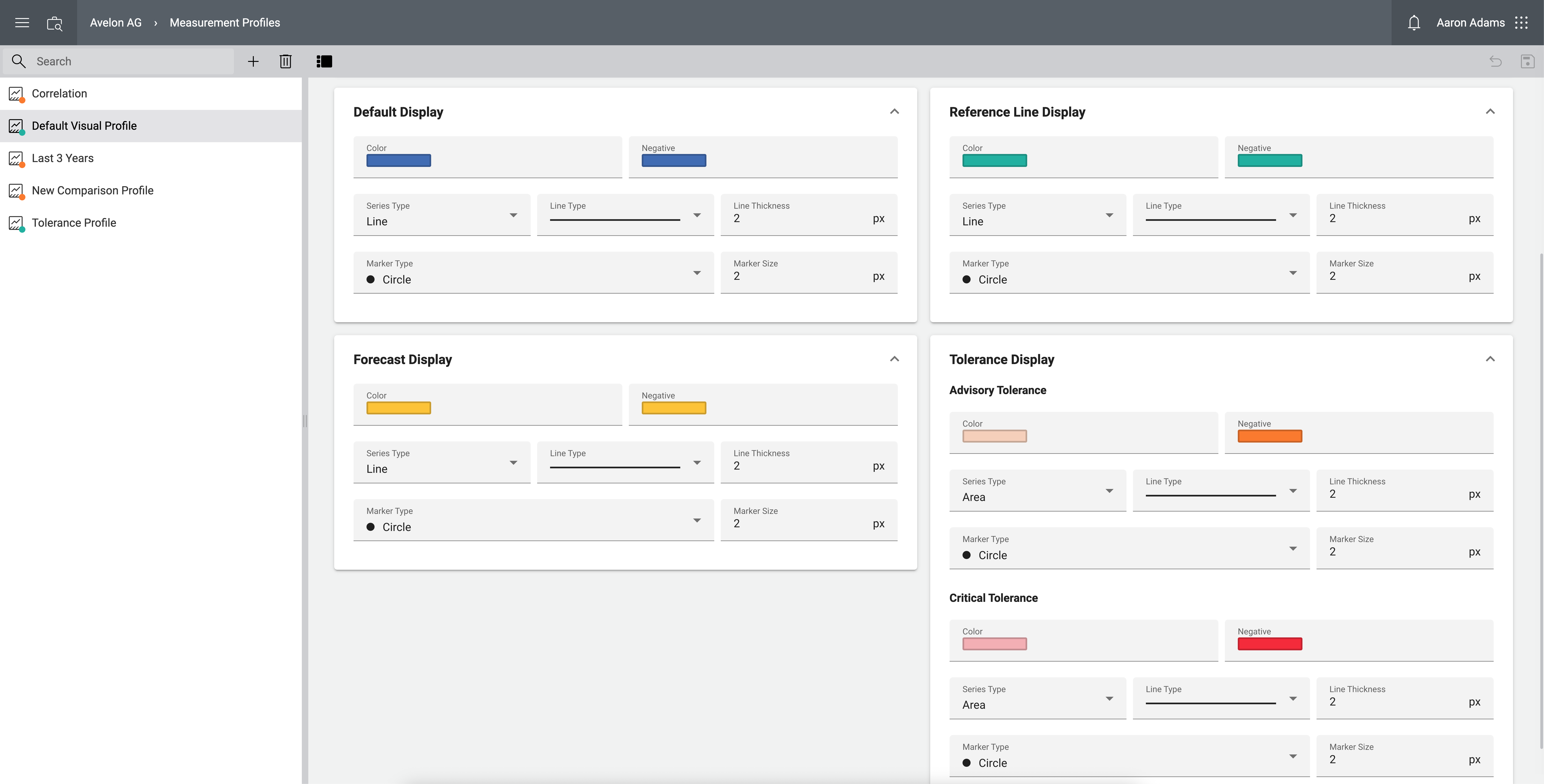
Visual profile

Define how individual aspects should be displayed in Chart widgets.

Stacking

Choose how this plot should be stacked when it’s displayed together with other data points with the same unit.

No stacking: Line plots overlap and column plots are displayed side by side.
Absolute: Plots are stacked on top of each other.
Relative: Plots are stacked on top of each other, relative to the sum of their values (= 100 %).

Default display

Determines how the plot should be displayed on the chart by default.

See visual settings below.

Reference line display

Determines how the reference line should be displayed on the chart by default.

See visual settings below.

Forecast display

Determines how the forecast should be displayed on the chart by default.

See visual settings below.

Tolerance display

Determines how the tolerances should be displayed on the chart by default.

See visual settings below.

Visual settings

Color

The color of the plot. This color is only applied to values that are greater or equal to 0.

Negative

The color of negative values.

Series Type

Specify how the plot should be displayed. The following types are available:

Line
Spline
Columns
Scatter
Area
Area Spline
Step Line Center
Step Line Left
Step Line Right

Line Type

The line style of the plot can be changed for the series types Line, Spline, Area, Area Spline and all Step Lines.

Line Thickness

The thickness of the line in pixels. Available for the series types Line, Spline, Area, Area Spline and all Step Lines.

Marker Type

The marker type that is displayed at the individual measuring points:

None
Circle
Square
Diamond
Triangle
Reversed Triangle

Marker Size

The size in pixels of the marker that was selected under Marker Type.

Comparison profile

On a comparison profile you can define how the system should calculate a reference line or a forecast.

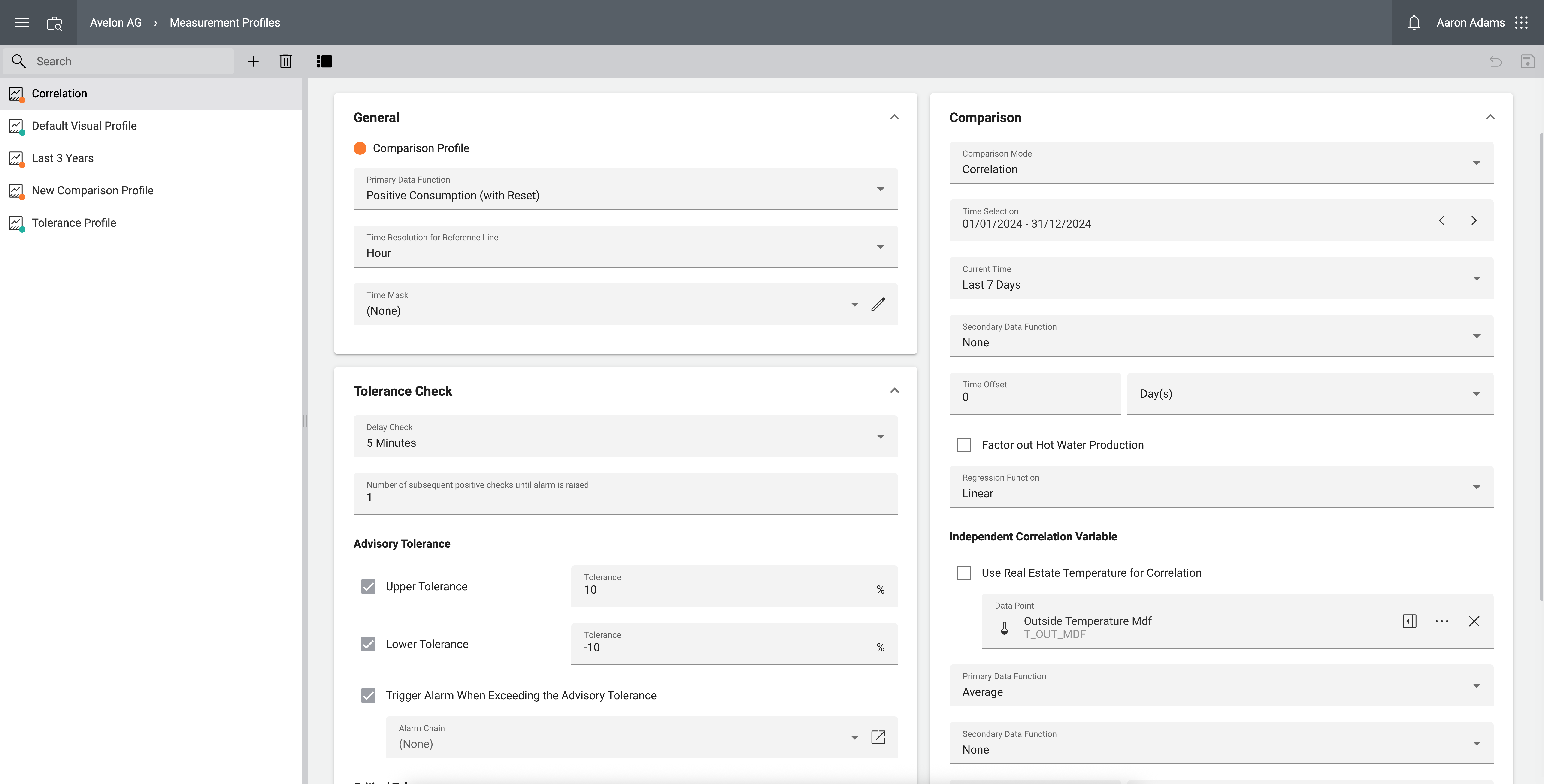
General

Primary Data Function

The primary function that is applied to the measurements of the data point for each aggregation interval. The aggregation interval is set in the field Time Resolution for Reference Line below.

Average
Minimum
Maximum
Sum
Positive Consumption
Positive Consumption (with Reset)
Negative Consumption
Positive and Negative Consumption

Time Resolution for Reference Line

The primary data function selected above will be applied to all values in every subsequent time interval with this length. This means that the reference line will only contain one value per interval according to the selected time resolution.

Minute
15 Minutes
Hour
Day
Week
Month
Quarter
Semester
Year
Quarter of Hour
Hour of Day
Day of Week
Day of Month
Day of Year
Day of Week in Month
Week of Year
Month of Year
Quarter of Year
Semester of Year

Note that some options might not be available, depending on the selected Comparison Mode (see below). For example, options with two units of time (e.g. day of week) are only available for the comparison mode Interval.

Time Mask

Only measurements within this time mask are taken into account for the calculation. If no time mask is configured, all measurements are taken into account.

Comparison

Comparison Mode

Value

With this comparison mode, the generated values for the reference line and the forecast are always constant.

Note that the comparison value is automatically converted to the unit of the data point to which the profile is applied.

The same constant value will be added to the reference line or forecast series for each aggregation interval according to the time resolution.

Comparison Value

Enter the static value with which the measurements should be compared.

Unit

The unit of the comparison value.

Note that the measurement profile can only be applied to data points that are compatible with this unit (i.e. data points with the same data type).

Interval

With this comparison mode, the reference line will be calculated as follows:

For each aggregation interval according to the Time Resolution, the system will determine the respective reference interval which comprises the last \(n\) complete comparison periods before the aggregation interval, and calculates the reference value using the primary data function over the values in that reference interval.

The calculation for forecast and reference line is identical, but for forecast the number of records that are taken into account will decrease the farther the calculation goes into the future.

If the time resolution consists of two units of time (e.g. hour of day), the inner unit is used as the time resolution (e.g. hour).

Note that forecast values are only calculated for the length of the comparison interval. For example, a comparison interval of 2 weeks will generate at most 2 weeks’ worth of data in the future.

Also note that the selected interval must be the same as the one selected in Time Resolution, or longer. If the time resolution consists of two units of time, the comparison interval must be at least the larger of the two units (e.g. if time resolution is “hour of day”, the comparison interval must be at least “day”).

Number of comparison intervals taken into account

Enter the number of comparison intervals that should be taken into account.

Comparison Interval

Select the comparison interval.

Year
Semester
Quarter
Month
Week
Day

Correlation

With this comparison mode, the reference line will be calculated as follows:

For each aggregation interval according to the Time Resolution, the system will

Calculate the reference interval according to the time selection for the start time of the aggregation interval.
Get the correlated values for the data point and the independent data point.
Calculate the model in the reference interval using the fitting strategy.
Use the value of the independent variable in the aggregation interval and plug it into the model to get the reference value.

The forecast will be calculated slightly differently:

The reference interval is calculated with respect to the current time, and a fixed model is calculated in that time that is valid for all future aggregation intervals.
The values for the independent variable are taken from the reference interval and plugged into the model. The individual aggregation intervals in the reference time interval are mapped to the future aggregation intervals.
If the reference interval is smaller than a year, the aggregation intervals are repeatedly mapped to the future aggregation intervals. Otherwise, the respective aggregation interval from last year is used instead. If the future period is larger than a year, the aggregation intervals are also mapped repeatedly.

Note that options with two units of time in Time Resolution are not supported for this comparison mode (e.g. day of week).

Time Selection

This time interval defines the reference interval. The reference line is calculated for the selected chart time interval.

Current Time

This is a time interval that is used to calculate the values that are used for the comparison.

Example: Assuming the time selection spans over one year and the current time is set to one month. The model will be calculated for the data of one year and applied to the last month resulting in reference values in the last month. These reference values are summed up and compared to the sum of the aggregated values (according to time resolution and primary data function) in that month.

Note that this has only an effect on the tolerance checks, but not on the reference line and forecast.

Secondary Data Function

The data function that is applied to the values which are returned by the primary data function.

None
Add Up
Difference

Time Offset

This time offset is applied to the measurement series of the source data point, which allows you to calculate the correlation between two different time intervals, e.g. today’s energy consumption and yesterday’s temperature.

Note that the independent correlation data point below can have its own time offset.

Factor out Hot Water Production

If this option is enabled, you can enter a hot water threshold. This threshold represents the independent value. Using the fitting model, the corresponding value is determined and subtracted from both values (reference value and original value) before calculating the deviation in percent.

The hot water threshold has to be entered in the same unit as the data point to which the profile is applied.

Note that this option only affects the tolerance check. Reference line and forecast are not affected by this option.

Regression Function

The regression function defines the fitting model between the two correlated variables. The model is used to calculate the reference line and forecast.

Linear
Segmented Linear
Polynomial
Exponential
Logarithmic

Independent Correlation Variable

Use Real Estate Temperature for Correlation

If this option is checked, the temperature data point that is currently set on the real estate will be used as the independent variable for the correlation analysis. This requires a temperature data point to be set on the real estate, which can be configured on the Real Estate Details widget under Climate Correction (Outside Temperature Difference) ▸ Reference Outside Temperature. Note that this temperature can only be set when the real estate has ESG/media reporting enabled, which requires an additional license “ESG/Media Reporting”.

If the real estate does not have a temperature data point set, or you want to use a different data point, just disable this option and select a custom data point in the Data Point field below.

Primary Data Function

The primary data function that is applied to the measurements of the independent correlation data point for each aggregation interval. The aggregation interval is set in the field Time Resolution for Reference Line in the card General.

Average
Minimum
Maximum
Sum
Positive Consumption
Positive Consumption (with Reset)
Negative Consumption
Positive and Negative Consumption

Secondary Data Function

The data function that is applied to the values which are returned for the independent correlation data point by the primary data function.

None
Add Up
Difference

Time Offset

This time offset is applied to the measurement series of the independent correlation data point, which allows you to calculate the correlation between two different time intervals, e.g. today’s energy consumption and yesterday’s temperature.

Note that the source data point of the measurement profile can have its own time offset, which can be configured above.

Time Mask

Only measurements from the independent correlation data point within this time mask are taken into account. If no time mask is configured, all measurements are taken into account.

Tolerance Check

Delay Check

Set the number of seconds to wait after the aggregation interval before the plausibility check is triggered.

The delay is needed because different devices send data at different intervals, or data might only be imported once per day. In some cases, the data might only be available a few hours after the corresponding interval has ended. For example, if the measurements are imported at 6 a.m. every day, the delay should be set to a value larger than 6 hours, e.g. 12 hours, so that the check runs after the data for the previous day has been imported.

5 Minutes
10 Minutes
30 Minutes
1 Hour
12 Hours
24 Hours

Number of subsequent positive checks until alarm is raised

The check has to be positive for this amount of times until an alarm is actually triggered.

Advisory Tolerance

Upper Tolerance: Enable and set the upper limit of the advisory tolerance.
Lower Tolerance: Enable and set the lower limit of the advisory tolerance.
Trigger Alarm When Exceeding the Advisory Tolerance: Enable this option to trigger a alarm when the value exceeds the upper advisory tolerance or falls below the lower advisory tolerance.

Critical Tolerance

Upper Tolerance: Enable and set the upper limit of the critical tolerance.
Lower Tolerance: Enable and set the lower limit of the critical tolerance.
Trigger Alarm When Exceeding the Critical Tolerance: Enable this option to trigger an alarm when the value exceeds the upper critical tolerance or falls below the lower critical tolerance.